Clouds 3: Skew – T and Instability

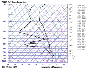
Figure 1: The skew-T diagram for 6 AM September 22, 2022, in Grand Junction, Colorado. From the University of Wyoming soundings archive.

Actual Temperature Profile: Environmental Lapse Rate

The actual local temperature profile is formally called the Environmental Lapse Rate (ELR). It is measured twice a day at specific locations all over the world, using weather balloons . Here in Colorado, this is done at the Grand Junction Airport. It was also done in Denver until July 2022 when a helium shortage required stopping the DEN service . The weather balloon carries a small, expendable instrument package called a radiosonde that transmits data to ground receiving stations. The data stream is called a ‘sounding’

Sounding Data

There are quite a few kinds of data transmitted by the radiosonde. For the purposes of understanding and identifying clouds, we are most interested in temperature, dewpoint and wind, all as a function of altitude. (Hang on, we’ll come back and define dewpoint in a bit.) Pressure and altitude are closely related, as we saw above, so we’ll treat them as interchangeable independent variables, and consider temperature, dewpoint and wind to be dependent on them. Usually when plotting functions you put the independent variable on the horizontal x-axis, and the dependent on the y-, but because we are talking about altitude, that will be on the y-axis. The units are both in meters and in millibars which vary inversely; the pressure goes down as the altitude goes up. The pressure units can be confusing: one bar is approximately one atmosphere of pressure, 14.7 psi, so sea level is around 1000 millibars. In SI units, one bar = 100,000 Pa (aka pascals or N/m2) or 100 kPa, but meteorologists prefer hPa, hectopascals, which are equal to millibars, the big blue vertical axis labels in Figure 1.   Anyways, the horizontal grid lines are thus isobars, lines of constant pressure. The altitude in meters is shown inside the axis. Temperature and dewpoint in centigrade will be on the x-axis, sort of. To keep a typical temperature profile looking good in a square format, the lines of constant temperature, isotherms, won’t be vertical, they will slant off to the right. That will make  a ‘Skew-T’ diagram, as shown in Figure 1. These diagrams are a bit complicated looking, and contain a lot of information. If you want to really get into it, you can take a free online short course in ‘Skew-T Mastery’ .

Figure 2: Skew-T, labeled. Skew-T diagrams can suggest where and what type of clouds are present. The altitude of clouds can be partially inferred by high relative humidity, where the dewpoint and temperature are close. The type of cloud is suggested by the stability of the atmosphere, determined by the steepness of the temperature profile compared to the adiabatic lapse rate. The underlying graph was downloaded from the University of Wyoming atmospheric soundings archive, http://weather.uwyo.edu/upperair/sounding.html. Annotations JeanBizHertzberg, 2022

Skew-T Plots

Skew-T diagrams have two primary lines. The heavy line on the right shows the air temperature recorded as the balloon ascends. If we are thinking about atmospheric stability, and whether a parcel rising from below is more or less dense than ‘the neighbors’, this line represents the environment, the temperature of the neighbors.

The heavy line on the left is the dewpoint. This is the temperature at which water vapor in the air at that height would condense into dew or a cloud. In other words, at the dewpoint the air holds its maximum possible amount of water vapor; we say the air is saturated. The dewpoint represents the amount of water vapor in the air: if the dewpoint is far from the actual local temperature, the air is relatively dry. If the dewpoint is close to the temperature line, the air doesn’t need to cool much before being saturated, and a cloud is likely to exist there. Another clue is that the temperature line will have a kink to the right. Condensation is ‘warming’ because thermal energy leaves the condensing water and enters the surrounding air; this will be seen in the temperature line angling closer to an isotherm. We are all familiar with the opposite effect since evaporating sweat cools our skin.

The stability of the atmosphere can be determined by the angle of the temperature line compared to an adiabat. Let’s use the moist adiabat for comparison if we are inside a cloud, or the dry adiabat if we are not. Here’s the procedure:

  1.  Choose a point on the temperature line. For example, let’s start near the ground. This defines the initial condition of our test parcel, our imaginary cube of air.
  2. Do a virtual lift of our parcel by moving a short distance upwards, parallel to the nearest dry adiabat line. We are thus perturbing our system by lifting our cube, and letting it cool adiabatically.
  3. Check to see if our lifted parcel is cooler — and more dense — or warmer — and less dense — than the actual (environmental) temperature line, representing its neighbors at that same height.
  4. Now let go of the parcel. Where does it go? If our parcel is cooler and denser, it will sink back down. This means the atmosphere is stable to perturbation; the lifted parcel drops back to where it came from. In contrast, if the parcel is warmer and less dense, it is buoyant and will keep going up! Unstable!

In summary, if the adiabat is shallower — less steep — than the temperature line, the atmosphere is stable. If the adiabat is steeper, it’s unstable. If the upper air is relatively cold — colder than adiabatic cooling makes it — and the air underneath is relatively warmer, we have an unstable situation. This happens often in summer because the sun heats the ground faster than it heats the air, and we get thunderstorms if there’s enough moisture in the air. In winter, the ground radiates a lot of heat to outer space on clear nights, making the air near the ground very cold — colder than the air aloft, i.e., a stable situation. This is called an inversion because it’s contrary to the normal adiabatic profile. This is a generality; weather has a lot of variety and is almost never ‘normal’!

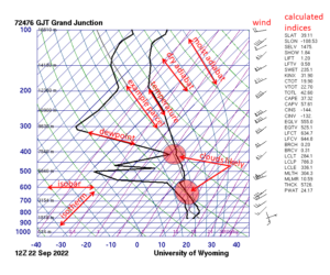
A shortcut to checking the whole column of the troposphere is to look at the CAPE (convective available potential energy), which can give us a good first guess on atmospheric stability (of course it’s more complicated than I’m showing here). On the right side of Figure 2 there is a column of ‘calculated indices’, quantities that have been computed from the data in the figure. Halfway down the column you’ll find CAPE, an integral of all the area between the adiabat and the temperature line where the adiabat is steeper. If CAPE is zero, the adiabat isn’t steeper than the temperature line anywhere, and the atmosphere is all stable, all the way up (more on clouds in stable air later).  A CAPE of a few hundred is weakly unstable, and small to medium (humulis, mediocris) cumulus clouds are expected. A CAPE of 1000 or more is very unstable and means that a thunderstorm is likely: cumulus congestus, cumulus castellanus and cumulonimbus will be seen. We see cauliflower-shaped cumulus in unstable air as the rising air essentially bubbles upwards, forming large buoyant turbulent jets .

Winds

Figure 3: Wind barb code from the National Weather Service.

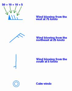
There is one more type of data on the Skew-T that is helpful in cloud ID, and that is the wind. Between the graph and the indices column there is a stack of feathers, called wind barbs. Figure 3 shows how to read the barbs. This is the standard code used by the National Weather Service when reporting data from weather stations and balloons. The wind speed is reported in knots which is a speed unit 15% faster than miles per hour. I usually ignore the difference. Knot is a very old nautical term which is still used for some navigation and weather data . Wind at altitudes above 300 mb (that’s millibar, not megabytes), in the upper half of the troposphere, are generally ‘westerly’; winds are named for where they are from, not where they are going. This altitude, 300 mb or 8-12 km up, seen in the upper quarter of the Skew-T, is where the jet stream flows from west to east in the northern hemisphere, although it wiggles around quite a bit. Note that the upper air winds are much faster than surface winds. The earth’s boundary layer effect slows and turns surface winds . The Skew-T tells you about winds vs altitude in a small region, but if you want to see both the jet stream and surface winds bringing you your weather in the near future, my current favorite app is Windy.com.

Wind can have a large effect on cloud development. For example, wind shear is when the speed or direction of the wind changes with altitude. This is common near the ground and up through the boundary layer to the ‘free atmosphere’ at a few hundred meters up. When there is wind shear higher up, it can prevent updrafts and downdrafts inside thunderstorms from canceling, and lead to severe thunderstorms storms with damaging hail that last for hours . Wind is also crucial in the formation of mountain wave clouds, discussed in Clouds 5: Lift Mechanism 2 – Orographics.

Figure 4: When downloading from the U Wyoming upper air archive, choose Skew-T GIF, date and time, then click on location. The image will open in a new browser tab.

How to Download a Skew-T

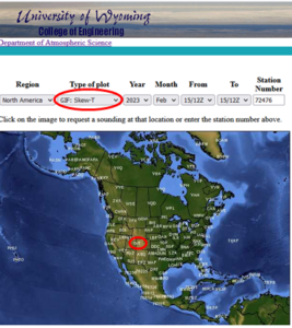
The best archive of Skew-T data for the US is maintained by the University of Wyoming: http://weather.uwyo.edu/upperair/sounding.html. The date and time are a bit tricky; they are specified in Universal Coordinated Time (UTC), a.k.a., Zulu military time (hence the Z) and Greenwich Mean Time (GMT), the date time at the prime meridian in England. Soundings are taken at 6 a.m. and 6 p.m. local time here in Colorado, so in the example shown in Figure 4, we can request the Skew-T plot for February 15 at 12Z, which is the one taken on Feb 15 at 6 a.m. here. The next sounding after that will be taken at 6 p.m., but it will be midnight on Feb 16 in England then, so we will have to request the Feb 16/00Z sounding.

References

[1]
“Non-Newtonian fluid,” Wikipedia. Aug. 06, 2024. Available: https://en.wikipedia.org/w/index.php?title=Non-Newtonian_fluid&oldid=1238844816#Oobleck. [Accessed: Aug. 07, 2024]
[1]
JeanBizHertzberg, English:  Consider a bubble in a curved streamline. Assume the bubble is small, but much less dense than the fluid. Let’s say the curved flow is in the horizontal plane - in other words, don’t worry about gravity making the particle fall just yet. Now, what will the bubble path look like compared to the fluid path? A) It will curve to the inside of the fluid streamline. B) It will track with the fluid. C) It will go straight along a tangent to the streamline. D) It will curve to the outside of the streamline. E) It will curve out away from the streamline. 2024. Available: https://commons.wikimedia.org/wiki/File:Bubble_path_in_a_fluid_question.png. [Accessed: Aug. 01, 2024]
[1]
“Upload Wizard - Wikimedia Commons.” Available: https://commons.wikimedia.org/wiki/Special:UploadWizard. [Accessed: Aug. 01, 2024]
[1]
JeanBizHertzberg, English:  Consider a particle in a curved streamline. Assume the particle is small, but much denser than the fluid. Let’s say the curved flow is in the horizontal plane - in other words, don’t worry about gravity making the particle fall just yet. Now, what will the particle path look like compared to the fluid path? A) It will curve to the inside of the fluid streamline. B) It will track with the fluid. C) It will go straight along a tangent to the streamline. D) It will curve to the outside of the streamline. E) It will curve out away from the streamline. 2024. Available: https://commons.wikimedia.org/wiki/File:Particle_path_in_a_fluid_question.png. [Accessed: Aug. 01, 2024]
[1]
World Meteorological Organization, “Cloud Atlas,” International Cloud Atlas. Available: https://cloudatlas.wmo.int/en/home.html. [Accessed: Mar. 29, 2023]
[1]
N. & U. A. F. J. T. H. / E. S. / M. J. O. / M. J. Vanderhal, English:  Air-to-air photography of a Northrop T-38 Talon in supersonic flight over the Mojave Desert reveals air density changes caused by flow regime transition around the aircraft, and the turbulent exhaust of the aircraft’s jet engines.This photo was acquired using a technique named Air-to-air Background-Oriented Schlieren (AirBOS). The process involves imaging with a high-speed camera mounted on the bottom of a Beechcraft B-200 King Air aircraft while the T-38C passes underneath. The pattern formed by the desert ground underneath the aircraft is filmed separately, and then removed digitally from the captured images during post-processing. This reveals the distortions created by the shockwaves, which result from the change in the air’s refractive index caused by density changes. 2015. Available: https://commons.wikimedia.org/wiki/File:Shockwave_pattern_around_a_T-38C_observed_with_Background-Oriented_Schlieren_photography_(1).jpg. [Accessed: Feb. 27, 2022]
[1]
L. K. Rajendran, J. Zhang, S. Bhattacharya, S. P. M. Bane, and P. P. Vlachos, “Uncertainty quantification in density estimation from background-oriented Schlieren measurements,” Meas. Sci. Technol., vol. 31, no. 5, p. 054002, Jan. 2020, doi: 10.1088/1361-6501/ab60c8. Available: https://dx.doi.org/10.1088/1361-6501/ab60c8. [Accessed: Aug. 07, 2023]
[1]
B. O. Cakir, S. Lavagnoli, B. H. Saracoglu, and C. Fureby, “Assessment and application of optical flow in background-oriented schlieren for compressible flows,” Exp Fluids, vol. 64, no. 1, p. 11, Dec. 2022, doi: 10.1007/s00348-022-03553-z. Available: https://doi.org/10.1007/s00348-022-03553-z. [Accessed: Aug. 07, 2023]
[1]
B. Mercier, S. Hamidouche, R. Gautier, and T. Lacassagne, “Educational Background Oriented Schlieren based on a Matlab App and a smartphone camera.,” 2022.
[1]
Bertrand Mercier, “comBOS: Open Matlab source for BOS,” Aug. 07, 2023. Available: https://www.mathworks.com/matlabcentral/fileexchange/111430-combos. [Accessed: Aug. 07, 2023]
[1]
“OpenPIV-BOS (Background Oriented Schlieren) by OpenPIV.” Available: http://www.openpiv.net/bos/. [Accessed: Aug. 07, 2023]
[1]
Lilly Verso and Alex Liberzon, Background Oriented Schlieren for stratified liquid cases. OpenPIV, 2023. Available: https://github.com/OpenPIV/bos. [Accessed: Aug. 07, 2023]
[1]
L. Verso and A. Liberzon, “Background oriented schlieren in a density stratified fluid,” Review of Scientific Instruments, vol. 86, no. 10, p. 103705, Oct. 2015, doi: 10.1063/1.4934576. Available: https://doi.org/10.1063/1.4934576. [Accessed: Aug. 07, 2023]
[1]
Gary Settles and Alex Liberzon, “Open Source BOS,” Tel Aviv University Turbulence Lab Open Source Projects. Available: https://www.turbulencelab.sites.tau.ac.il/projects-6. [Accessed: Aug. 07, 2023]
[1]
NathanHagen, English:  Optical layout of a single-mirror schlieren system. 2022. Available: https://commons.wikimedia.org/wiki/File:Single_mirror_schlieren.svg. [Accessed: Aug. 04, 2023]
[1]
NathanHagen, English:  Optical layout of a two-mirror schlieren system, showing only the undeviated rays. 2022. Available: https://commons.wikimedia.org/wiki/File:Double_mirror_schlieren_layout.svg. [Accessed: Aug. 03, 2023]
[1]
“SCHLIEREN PHOTOGRAPHY PRINCIPLES.” Available: https://people.rit.edu/andpph/text-schlieren.html. [Accessed: Aug. 01, 2023]
[1]
“Schlieren Optics.” Available: https://sciencedemonstrations.fas.harvard.edu/presentations/schlieren-optics. [Accessed: Aug. 01, 2023]
[1]
“Schlieren photography,” Wikipedia. Apr. 09, 2023. Available: https://en.wikipedia.org/w/index.php?title=Schlieren_photography&oldid=1148932520. [Accessed: Aug. 01, 2023]
[1]
W. Merzkirch, Flow Visualization, Second Edition, 2nd ed. Academic Press, 1987.
[1]
H. Fiedler, K. Nottmeyer, P. P. Wegener, and S. Raghu, “Schlieren photography of water flow,” Experiments in Fluids, vol. 3, no. 3, pp. 145–151, May 1985, doi: 10.1007/BF00280452. Available: https://doi.org/10.1007/BF00280452. [Accessed: Jul. 25, 2023]
[1]
R. E. Bland and T. J. Pelick, “The Schlieren Method Applied to Flow Visualization in a Water Tunnel,” Journal of Basic Engineering, vol. 84, no. 4, pp. 587–592, Dec. 1962, doi: 10.1115/1.3658718. Available: https://doi.org/10.1115/1.3658718. [Accessed: Jul. 25, 2023]
[1]
C. Isenberg, The science of soap films and soap bubbles. New York: Dover Publications, 1992.
[1]
R. Bruinsma, “Theory of hydrodynamic convection in soap films,” Physica A: Statistical Mechanics and its Applications, vol. 216, no. 1, pp. 59–76, Jun. 1995, doi: 10.1016/0378-4371(95)00023-Z. Available: https://www.sciencedirect.com/science/article/pii/037843719500023Z. [Accessed: Jul. 24, 2023]
[1]
FlowVis@CU, “A horizontal soap bubble film drains towards its center, while nonuniformities from undissolved sugar crystals create colored patterns as the film thickness varies.,” Flow Visualization, May 21, 2015. Available: https://www.flowvis.org/2015/05/21/a-horizontal-soap-bubble-film-drains-towards-its-center-while-nonuniformities-from-undissolved-sugar-crystals-create-colored-patterns-as-the-film-thickness-varies/. [Accessed: Jul. 24, 2023]
[1]
“Wave interference,” Wikipedia. Jun. 29, 2023. Available: https://en.wikipedia.org/w/index.php?title=Wave_interference&oldid=1162450191. [Accessed: Jul. 24, 2023]
[1]
Z. Sándor, Magyar:  Fénytörés. 2005. Available: https://commons.wikimedia.org/wiki/File:F%C3%A9nyt%C3%B6r%C3%A9s.jpg. [Accessed: Jul. 24, 2023]
[1]
Nicoguaro, English:  A wave of light reflecting off the upper and lower boundaries of a thin film. 2016. Available: https://commons.wikimedia.org/wiki/File:Thin_film_interference.svg. [Accessed: Jul. 19, 2023]
[1]
“Thin-film interference,” Wikipedia. May 10, 2023. Available: https://en.wikipedia.org/w/index.php?title=Thin-film_interference&oldid=1154105139. [Accessed: Jul. 18, 2023]
[1]
D. P. B. Smith, English:  Shadowgraph of bullet in flight. 1962. Available: https://commons.wikimedia.org/wiki/File:Shockwave.jpg. [Accessed: Jul. 18, 2023]
[1]
“Shadowgraphy (performing art),” Wikipedia. Mar. 17, 2023. Available: https://en.wikipedia.org/w/index.php?title=Shadowgraphy_(performing_art)&oldid=1145180624. [Accessed: Jul. 18, 2023]
[1]
“Optical properties of water and ice,” Wikipedia. Feb. 19, 2023. Available: https://en.wikipedia.org/w/index.php?title=Optical_properties_of_water_and_ice&oldid=1140373202. [Accessed: Jul. 18, 2023]
[1]
“Dispersion (optics),” Wikipedia. Jun. 21, 2023. Available: https://en.wikipedia.org/w/index.php?title=Dispersion_(optics)&oldid=1161233581. [Accessed: Jul. 17, 2023]
[1]
FlowVis@CU, “Sunlight is concentrated into ‘caustics’ by small waves on the water surface, here near a Caribbean beach.,” Flow Visualization, Nov. 09, 2014. Available: https://www.flowvis.org/2014/11/09/sunlight-is-concentrated-into-caustics-by-small-waves-on-the-water-surface-here-near-a-caribbean-beach-2/. [Accessed: Jul. 17, 2023]
[1]
J. Bertolotti, Caustics gif. 2020. Available: https://commons.wikimedia.org/wiki/File:Caustics.gif. [Accessed: Jul. 17, 2023]
[1]
“Caustic (optics),” Wikipedia. Apr. 10, 2023. Available: https://en.wikipedia.org/w/index.php?title=Caustic_(optics)&oldid=1149188519. [Accessed: Jul. 17, 2023]
[1]
“Shadowgraph,” Wikipedia. May 05, 2023. Available: https://en.wikipedia.org/w/index.php?title=Shadowgraph&oldid=1153358078. [Accessed: Jul. 17, 2023]
[1]
H. Wang, “From Contact Line Structures to Wetting Dynamics,” Langmuir, vol. 35, no. 32, pp. 10233–10245, Aug. 2019, doi: 10.1021/acs.langmuir.9b00294. Available: https://doi.org/10.1021/acs.langmuir.9b00294. [Accessed: Jul. 16, 2023]
[1]
“Reflectance,” Wikipedia. May 23, 2023. Available: https://en.wikipedia.org/w/index.php?title=Reflectance&oldid=1156571917. [Accessed: Jul. 16, 2023]
[1]
FlowVis@CU, “Light reflects from standing waves on the surface of water in an ultrasonic cleaner.,” Flow Visualization, Feb. 24, 2013. Available: https://www.flowvis.org/2013/02/24/light-reflects-from-standing-waves-on-the-surface-of-water-in-an-ultrasonic-cleaner/. [Accessed: Jul. 16, 2023]
[1]
Dan Pangburn, “File:Water reflectivity.jpg,” Wikipedia. Mar. 22, 2012. Available: https://en.wikipedia.org/w/index.php?title=File:Water_reflectivity.jpg&oldid=483290200. [Accessed: Jul. 14, 2023]
[1]
Fermilab, Why does light slow down in water?, (Feb. 20, 2019). Available: https://www.youtube.com/watch?v=CUjt36SD3h8. [Accessed: Jul. 13, 2023]
[1]
M. Lloyd, “Michael Lloyd: Clouds First,” Flow Visualization, Oct. 01, 2016. Available: https://www.flowvis.org/2016/10/01/michael-lloyd-clouds-first/. [Accessed: Jul. 11, 2023]
[1]
“Rayleigh–Bénard convection,” Wikipedia. May 04, 2023. Available: https://en.wikipedia.org/w/index.php?title=Rayleigh%E2%80%93B%C3%A9nard_convection&oldid=1153087302. [Accessed: Jul. 10, 2023]
[1]
R. A. Houze, “Clouds in Shallow Layers at Low, Middle, and High Levels,” in Cloud Dynamics, in International Geophysics, vol. 104. Elsevier, 2014, pp. 125–127. doi: 10.1016/B978-0-12-374266-7.00005-6. Available: https://linkinghub.elsevier.com/retrieve/pii/B9780123742667000056. [Accessed: Jul. 10, 2023]
[1]
FlowVis@CU, “Altostratus lenticularis, 2/18/14, 5:15 pm,” Flow Visualization, Apr. 06, 2014. Available: https://www.flowvis.org/2014/04/06/altostratus-lenticularis-2-18-14-515-pm/. [Accessed: Jul. 10, 2023]
[1]
FlowVis@CU, “A persistent spreading contrail below altostratus, color reversed, Boulder CO, March 11, 2013 at 3:45 pm.,” Flow Visualization, Sep. 07, 2013. Available: https://www.flowvis.org/2013/09/07/a-persistent-spreading-contrail-below-altostratus-color-reversed-boulder-co-march-11-2013-at-345-pm/. [Accessed: Jul. 10, 2023]
[1]
FlowVis@CU, “Altostratus at dawn, Louisville CO, February 17th 2013 at about 6:40 a.m.,” Flow Visualization, Sep. 03, 2013. Available: https://www.flowvis.org/2013/09/03/altostratus-at-dawn-louisville-co-february-17th-2013-at-about-640-a-m/. [Accessed: Jul. 10, 2023]
[1]
FlowVis@CU, “A persistent spreading contrail below altostratus, color reversed, Boulder CO, March 11, 2013 at 3:45 pm.,” Flow Visualization, Sep. 07, 2013. Available: https://www.flowvis.org/2013/09/07/a-persistent-spreading-contrail-below-altostratus-color-reversed-boulder-co-march-11-2013-at-345-pm/. [Accessed: Jul. 05, 2023]
[1]
“COLD FRONT - Meteorological Physical Background.” Available: https://rammb.cira.colostate.edu/wmovl/vrl/tutorials/satmanu-eumetsat/satmanu/cms/cf/backgr.htm. [Accessed: Jul. 05, 2023]
Clouds 2: Why Are There Clouds? Lift Mechanism 1: Instability
Clouds 4: Clouds in Unstable Atmosphere